STATISTICAL
INFERENCE
In this part we will use the Summerton sales as a basis
for predicting property values in that suburb.
See analyzing and
presenting data
The use of predicted
sale prices is not so much a valuation method (as this is not
acceptable to the courts or industry) but as a description of possible
trends in this locality. That is, as with the previous part sales data
can be analyzed and used to predict general values in foe example, an
"investment report".
CONFIDENCE INTERVALS
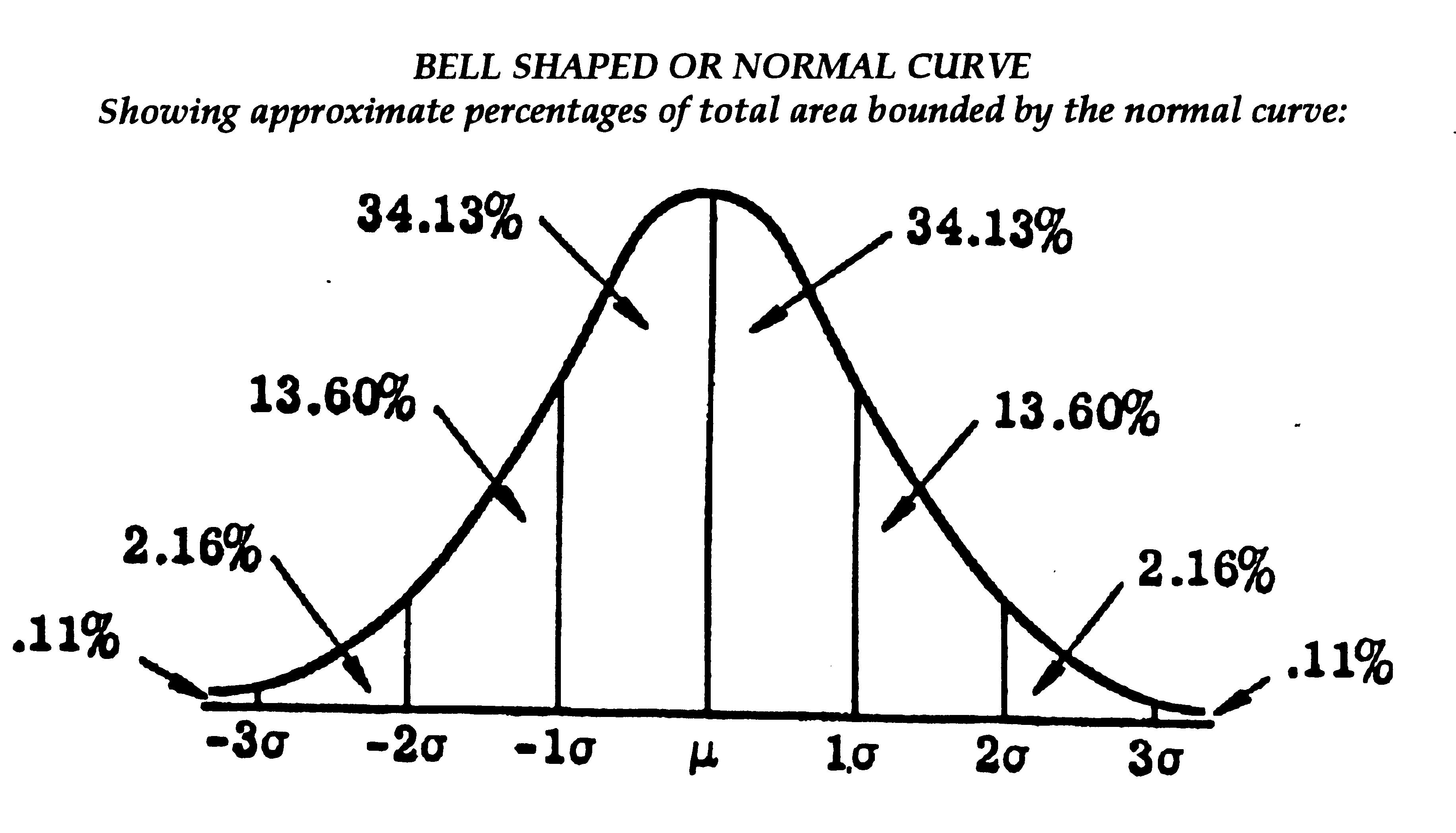
The standard
deviation can be used to indicate what percentage of the sample of a
population may be expected to fall within selected confidence
intervals. As the diagram below shows about 68.26% of the sample of the
population will generally fall within plus or minus one standard
deviation from the mean assuming that the data approximates a normal
distribution.
Normally at least 30 random sales are required to confidently state
that the sample is representative of the population. For Summerton we
only have 19 sales which are skewed, but for the purposes of this part
we will assume that the sample approximates a normal curve and is
representative of the population (Summerton houses).
Assuming the sales
data in Summerton approximates a normal distribution 68.26% of the
sales will fall between the mean - 1 standard deviation and the mean +
1 standard deviation, about 95.44% should fall with 2 standard
deviations either side of the mean and about 99.74% should fall within
3 standard deviations either side of the mean - see diagram above.
STATISTICAL INFERENCE
Past sale prices and rents can be used to predict future prices, rents,
and values.
EXAMPLE
What percentage of sales fall within the range of 10 (000) on either
side of the mean (598.4) for the Summerton sales?
Using the Z score formula:
Z = R/STD = 10/325.5 = 0.0307
Where:
R = required range (10)
STD = standard deviation
The Z score shows that 608.4 and 588.4 each deviate from the mean by
0.0307 standard deviations. The percent is found by referring to the
diagram below which shows a value of about 0.012. Therefore, about 1.2%
of sales lie between the mean and 608.4 and about 2.4% lie between
608.4 and 588.4.
PROBABILITY
USING Z VALUES
The probability of a
selected sale falling between a given range can be found with the above
formula. For a range of +5(000) and -5(000) of either side of the mean:
Z = 5/325.5 = 0.0154
See Z values – table
The Z value table shows that a Z value of 0.0154 corresponds to about
.006 (by interpolation) Therefore, there is about a 0.6% chance that
the sale will fall within the range 5(000) above the mean or 1.2%
chance that it will fall between 330.5 and 320.5.
CONFIDENCE LEVELS
For a number of
statistical analyses a 95% confidence level is required. From the
previous calculations we can state with 95% degree of confidence a sale
will fall between 1.96 standard deviations either side of the mean -
see diagram above and Z value table.
That is 1.96 * 325.5
= 638 either side of the mean however, such statements depend on how
accurately the estimated mean represents the population mean.
Regardless of the size of the population there is a specific sample
size that will permit a certain level of confidence in the estimated
mean.
NECESSARY SAMPLE SIZE
The necessary sample
size can be calculated with the following formula:
n = (Z2*STD2)/e2
Where:
n = the sample size required
z = z value at the required degree of confidence eg 95%
STD = standard deviation
e = range from the
mean.
EXAMPLE
Determine the sample size required from Summerton for the valuer to be
95% confident that the true mean is within +/-10(000) of the estimated
mean of 600(000). That is, between 588.4 and 608.4(000):
n = (1.962*325.52)/102 = (3.842 * 105950)/100 = 407061/100 = 4071
Therefore, the
Summerton sample is well short of the required number of sales for the
valuer to be 95% confident that they will represent the population.
Note that this confidence limit is at variance with standard valuation
practice where commonly, a few comparable sales meeting the rigorous
standards of the willing buyer-willing seller theory will
provide extremely reliable evidence of market value.
SCATTERPLOTS
Scatterplots are
useful devices for determining relationships between variables. In
valuation work there are a number of variables which affect the value
of real estate which can be shown to correlate with market value.
EXAMPLE
The 19 sales in
Summerton are plotted against distance from the local railway station.
The following scatterplot results:
SALE PRICE VERSUS
DISTANCE FROM RAILWAY STATION
A visual inspection
of the scatterplot above shows a reasonable inverse correlation between
sale prices and distance from the local railway station. On the other
hand the scatterplot below shows no discernable pattern and there would
appear to be no correlation between sale price and distance from
railway station:
OUTLIERS
There are 2 or 3
outliers shown on the scatterplot. Outliers are most important and will
show either an error in the sample or application or may indicate an
interesting new variable which should be examined. Valid outliers
require further investigation.
Upon investigation it
is found that the reason why prices of the outliers had held up so well
despite the distance from the local railway station is because they
come inside the commuting area of the neighbouring railway station.
Therefore, the plot would support the hypothesis.
TIME SERIES
Values and rents can
be traced over time to ascertain a trend and for prediction. Although
cyclical theory has been discredited for land values the "boom bust"
pattern can be discerned over time.
STATISTICAL
INFERENCE
In this part we will use the Summerton sales as a basis
for predicting property values in that suburb.
See analyzing and
presenting data
The use of predicted
sale prices is not so much a valuation method (as this is not
acceptable to the courts or industry) but as a description of possible
trends in this locality. That is, as with the previous part sales data
can be analyzed and used to predict general values in foe example, an
"investment report".
CONFIDENCE INTERVALS
The standard
deviation can be used to indicate what percentage of the sample of a
population may be expected to fall within selected confidence
intervals. As the diagram below shows about 68.26% of the sample of the
population will generally fall within plus or minus one standard
deviation from the mean assuming that the data approximates a normal
distribution.
Normally at least 30 random sales are required to confidently state
that the sample is representative of the population. For Summerton we
only have 19 sales which are skewed, but for the purposes of this part
we will assume that the sample approximates a normal curve and is
representative of the population (Summerton houses).
Assuming the sales
data in Summerton approximates a normal distribution 68.26% of the
sales will fall between the mean - 1 standard deviation and the mean +
1 standard deviation, about 95.44% should fall with 2 standard
deviations either side of the mean and about 99.74% should fall within
3 standard deviations either side of the mean - see diagram above.
STATISTICAL INFERENCE
Past sale prices and rents can be used to predict future prices, rents,
and values.
EXAMPLE
What percentage of sales fall within the range of 10 (000) on either
side of the mean (598.4) for the Summerton sales?
Using the Z score formula:
Z = R/STD = 10/325.5 = 0.0307
Where:
R = required range (10)
STD = standard deviation
The Z score shows that 608.4 and 588.4 each deviate from the mean by
0.0307 standard deviations. The percent is found by referring to the
diagram below which shows a value of about 0.012. Therefore, about 1.2%
of sales lie between the mean and 608.4 and about 2.4% lie between
608.4 and 588.4.
PROBABILITY
USING Z VALUES
The probability of a
selected sale falling between a given range can be found with the above
formula. For a range of +5(000) and -5(000) of either side of the mean:
Z = 5/325.5 = 0.0154
See Z values – table
The Z value table shows that a Z value of 0.0154 corresponds to about
.006 (by interpolation) Therefore, there is about a 0.6% chance that
the sale will fall within the range 5(000) above the mean or 1.2%
chance that it will fall between 330.5 and 320.5.
CONFIDENCE LEVELS
For a number of
statistical analyses a 95% confidence level is required. From the
previous calculations we can state with 95% degree of confidence a sale
will fall between 1.96 standard deviations either side of the mean -
see diagram above and Z value table.
That is 1.96 * 325.5
= 638 either side of the mean however, such statements depend on how
accurately the estimated mean represents the population mean.
Regardless of the size of the population there is a specific sample
size that will permit a certain level of confidence in the estimated
mean.
NECESSARY SAMPLE SIZE
The necessary sample
size can be calculated with the following formula:
n = (Z2*STD2)/e2
Where:
n = the sample size required
z = z value at the required degree of confidence eg 95%
STD = standard deviation
e = range from the
mean.
EXAMPLE
Determine the sample size required from Summerton for the valuer to be
95% confident that the true mean is within +/-10(000) of the estimated
mean of 600(000). That is, between 588.4 and 608.4(000):
n = (1.962*325.52)/102 = (3.842 * 105950)/100 = 407061/100 = 4071
Therefore, the
Summerton sample is well short of the required number of sales for the
valuer to be 95% confident that they will represent the population.
Note that this confidence limit is at variance with standard valuation
practice where commonly, a few comparable sales meeting the rigorous
standards of the willing buyer-willing seller theory will
provide extremely reliable evidence of market value.
SCATTERPLOTS
Scatterplots are
useful devices for determining relationships between variables. In
valuation work there are a number of variables which affect the value
of real estate which can be shown to correlate with market value.
EXAMPLE
The 19 sales in
Summerton are plotted against distance from the local railway station.
The following scatterplot results:
SALE PRICE VERSUS
DISTANCE FROM RAILWAY STATION
A visual inspection
of the scatterplot above shows a reasonable inverse correlation between
sale prices and distance from the local railway station. On the other
hand the scatterplot below shows no discernable pattern and there would
appear to be no correlation between sale price and distance from
railway station:
OUTLIERS
There are 2 or 3
outliers shown on the scatterplot. Outliers are most important and will
show either an error in the sample or application or may indicate an
interesting new variable which should be examined. Valid outliers
require further investigation.
Upon investigation it
is found that the reason why prices of the outliers had held up so well
despite the distance from the local railway station is because they
come inside the commuting area of the neighbouring railway station.
Therefore, the plot would support the hypothesis.
TIME SERIES
Values and rents can
be traced over time to ascertain a trend and for prediction. Although
cyclical theory has been discredited for land values the "boom bust"
pattern can be discerned over time.
The above time series
show office rents for a particular type of office block in Sydney over
a period of 5 years. The series can be made into a "control chart" by
including "upper" and "lower" control limits which are usually 2
standard deviations. These are shown on the Z value table and those
values outside the control limits are treated as outliers.
Often such plots need
smoothing to ascertain some underlining trend. This can be done
for example by using a running medium of 3 which means each
data point is the mean of that point plus its two neighbouring points.
"t" DISTRIBUTION
As sample sizes decrease the sampling distribution of their means
becomes more pointed in the middle and has relatively more area in
their tails. Such a distribution is known as the "t" distribution or
"students" distribution. The diagram below compares the normal curve A
with two "t" distributions, B and C:
THE "t" DISTRIBUTION VERSUS THE NORMAL CURVE
7