SENSITIVITY
ANALYSIS
All feasibility studies and valuations using the DCF approach to
measure the rate of return should be subject to a sensitivity analysis.
This will determine the most important variables in the cash flow and
show their comparative rate of change. The normal sensitivity analysis
adjusts the subject variable by +/- 10%. The resulting NPV or IRR using
the equated yield model is recorded in a table or on a graph to show
the sensitivity in terms of absolute amounts or slope of line. All
other variables are held equal. The most commonly analyzed variables
are:
FEASIBILITY STUDIES
Purchase price
or land value
Cost of
construction
Length of
development period
End market
value
EXISTING INVESTMENT
PROPERTIES
Purchase price
End market
value
Rental income
(this can also be use to measure different vacancy rates).
End market
value + rental income.
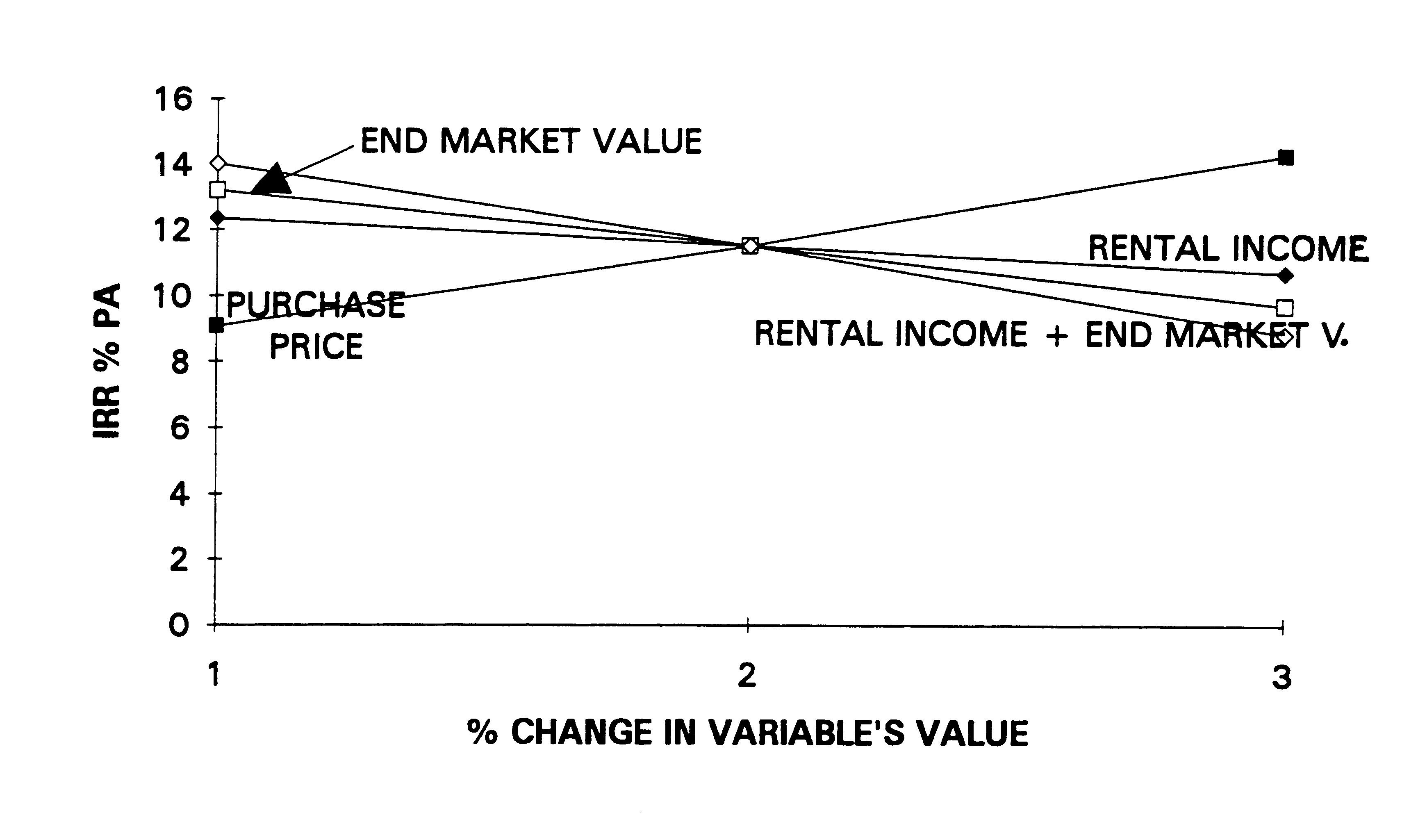
TABLESENSITIVITY ANALYSIS
FOR AN INVESTMENT REPORT OVER SUBJECT PROPERTY The
equated yield rates of return are used to determine the investment's
sensitivity:
VARIABLE VALUE CHANGE
+10%
-10%
PURCHASE PRICE:
9.08%
14.28%
END MARKET VALUE:
13.20%
9.69%
RENTAL INCOME ONLY:
12.34%
10.68%
RENTAL INCOME + END MARKET VALUE:
14.01%
8.83%
The
sensitivity analysis shows that the risk to investment is greatest with
a change in rental income which in turn affects the expected end market
value. The next most important single variable is the purchase price
which is slightly more sensitive than the end market value. Rental
income during the 5 year period is not a very sensitive variable at
all. The above results are better shown on a graph where the
sensitivity of each variable can be observed by it's slope. The steeper
the slope, the more sensitive is the variable - see diagram below:
DIAGRAMSLOPES OF VARIABLES -
SENSITIVITY ANALYSIS
SCENARIOS As
the sensitivity analysis shows, forecasting error can effect both the
feasibility of a project or the value of an existing building.
Therefore, in any situation where the result or value will vary greatly
due to forecasting error it is better for the valuer not to determine a
final answer but instead, provide 3 answers according to the following
scenarios:
Expected (E)
Optimistic (O)
Pessimistic (P)
EXPECTED SCENARIO
The expected scenario is the market's forecast that is, the cash flow
is constructed using data analysed from comparable sales. Where land
values are determined from such a DCF they are market values.
OPTIMISTIC SCENARIO
The optimistic
scenario is that cash flow constructed according to a 10% increase in
rental income and expected end market value. Therefore, the optimistic
scenario in the DCF will determine the highest land value, above market
value.
PESSIMISTIC SCENARIO
The pessimistic scenario is that cash flow which incorporates a 10%
decrease in rental income and expected end market value. Therefore, the
pessimistic scenario will provide the lowest land value, below market
value.Some valuers combine
a number of variable changes in the scenario for example, purchase
price, rental income and end market value. However, this can result in
scenarios which are extremely unlikely and will determine extreme
values.A single statistic
can be calculated for comparison purposes by using the PERT formula: