| NUMBER | TOTAL FIXED COST‘000 | TOTAL VARIABLE COST‘000 | TOTAL COST
'000 |
| 1 | 50 | 30 | 80 |
| 2 | 50 | 37 | 87 |
| 3 | 50 | 43 | 93 |
| 4 | 50 | 50 | 100 |
| 5 | 50 | 60 | 110 |
| 6 | 50 | 72 | 122 |
| 7 | 50 | 87 | 137 |
| 8 | 50 | 106 | 156 |
| 9 | 50 | 131 | 181 |
| 10 | 50 | 161 | 211 |
| VARIABLE INPUT
(LABOUR) |
$ VALUE OF VARIABLE
INPUT (LABOUR) ‘000 |
$ VALUE OF FIXED INPUT
(MAN’MENT) ‘000 |
TOTAL INPUT
(TOTAL COST) ‘000 |
COMMODITY
(HOUSES) |
| 5 | 150 | 180 | 330 | 1 |
| 11 | 200 | 180 | 380 | 2 |
| 17 | 255 | 180 | 435 | 3 |
| 23 | 310 | 180 | 490 | 4 |
| 30 | 370 | 180 | 550 | 5 |
| 37 | 430 | 180 | 610 | 6 |
| 45 | 495 | 180 | 675 | 7 |
| 55 | 565 | 180 | 745 | 8 |
| 66 | 640 | 180 | 820 | 9 |
|
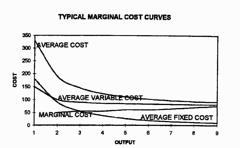
QUANTITY (HOUSES) |
AVERAGE COST (COST PER HOUSE) ‘000 |
MARGINAL COST ‘000 |
|
1 |
330 |
50 |
|
2 |
190 |
55 |
|
3 |
145 |
55 |
|
4 |
122.5 |
60 |
|
5 |
110 |
60 |
|
6 |
101.7 |
65 |
|
7 |
96.4 |
70 |
|
8 |
93.1 |
75 |
|
9 |
91.1 |
|